In the previous section, we discussed the Deutsch Algorithm. Here, we will talk about the Deutsch-Jozsa Algorithm. The differences between them will be discussed in depth in the next section. For now, our primary goal is to introduce the Deutsch-Jozsa Algorithm.

Let us start by explaining what this algorithm is. The Deutsch-Jozsa Algorithm is a quantum algorithm designed to determine whether a function is constant or balanced, specifically for classical computers. Since we discussed the concepts of constant and balanced functions in the previous section, we will not repeat them here. For classical computers, determining whether the function ( f ) is constant or balanced may require up to ( 2ⁿ ) evaluations. However, the Deutsch-Jozsa Algorithm achieves the correct result with only a single query.

As previously discussed, we have already defined constant and balanced functions in detail. Here, as a brief reminder, we can define them again. A classical function is constant if it produces the same output for every input. If the outputs differ for any two inputs, the function is balanced.

6.5.1. Algorithm Steps and Mathematical Details

a. Initial State

The algorithm works for an n -bit input function f: Bⁿ → B , where B = {0, 1} is the set of values each bit can take, either 0 or 1. Initially, the quantum state below is prepared:

• The first n-qubits are initialized in the |0⟩ state (i.e., the zero state).
• The last qubit is initialized in the |1⟩ state.

In this setup, there are a total of 2ⁿ possible states, as each qubit can be either 0 or 1. However, the last qubit is fixed in the |1⟩ state.

6.5.2. Hadamard Transformation

Initially, we apply the Hadamard transformation to both components of the system. The Hadamard transformation puts a qubit into a superposition state. For a single qubit, the Hadamard transformation is defined as:

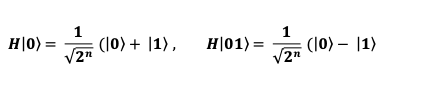
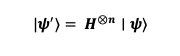
Applying the Hadamard transform to both qubits, the quantum state is as follows

This is a superposition state where all qubits are equally likely to be in both states 0 and 1. Now, we start to get information about the function 𝒇(𝒙).

6.5.3. Oracle Application (Oracle Gateway)

The function f is presented as a quantum oracle. The oracle takes the input state |x⟩ and transforms it into the state |x⟩ ⊗ f(x). In other words, it adds the value of f(x). When the oracle is applied to |𝝍⟩ , it produces the following state:

Here, for each x, 𝒇(𝒙) can be either 0 or 1. This step of the Oracle adds the state to 𝒇(𝒙) and provides our quantum computer with the information of the function 𝒇.

6.5.4. Subsequent Transformation

At this point, based on the information provided by the oracle, we apply another Hadamard transformation. This helps us determine the outcome of the function. After applying the Hadamard transformation to each qubit, the resulting state is:

This transformation allows us to gain more information about the system’s state. If f is constant, we will observe the result |00⟩. If f is balanced, the result could be |01⟩, |10⟩, or |11⟩.

6.5.5. Measurement

Finally, we measure the quantum state. If the system collapses to the |00⟩ state, the function is constant. If it collapses to one of the states |01⟩, |10⟩, or |11⟩, the function is balanced. This measurement process is used to determine the nature of the function and is significantly faster than classical algorithms. While classical algorithms require querying each input, the Deutsch-Jozsa algorithm achieves the result with a single query.

In summary:

• Initial State: An n-bit superposition is created.
• Hadamard Transformation: Hadamard gates are applied to the qubits.
• Oracle Application: The function f(x) is integrated into the system using an oracle.
• Final Transformation: The Hadamard transformation is applied again.
• Measurement: The function is determined to be either constant or balanced.

As a result of these steps, it is possible to determine whether f(x) is constant or balanced with only one query. In contrast, classical computers may require 2ⁿ queries for this task.